Quantitative Futures, stocks and Options Trading (AVAILABLE FOR MATLAB FREELANCING): 11/16/08

Sample Size equation that is predicated on Central Limit Theorem

Correction Factor for Sample Size based on finite Population Size

For a 95% Level, Z = 1.96. Let us say that we want the result to be within 5% error--Confidence Interval and lets have P varying
from 0.1 to 0.9. Then inserting the above numbers into the equation, we get:
ConfidenceInterval = 0.05;Z = 1.96;

P = 0.1:0.1:0.9;
SampleSize = [Z^2 .* P .* (1-P)]/(ConfidenceInterval^2);
SampleSizeRequired = [P ;SampleSize].'
SampleSizeRequired =
0.1000 138.2976
0.2000 245.8624
0.3000 322.6944
0.4000 368.7936
0.5000 384.1600
0.6000 368.7936
0.7000 322.6944
0.8000 245.8624
0.9000 138.2976

Plot of SampleSize Required vs Probability:

figure()

plot(SampleSizeRequired(:,1),SampleSizeRequired(:,2))

xlabel('Probability P')

ylabel('Sample Size Required')

T-distribution table VS Sample Size and closeness to Standard Normal:

(Source: Jeffrey Russell NOTES)

T distribution with n-1 degrees of freedom at 0.05 level( 95%) It becomes normal when T is Approx 2 ( 1.96 to be exact)

% T     n

[4.303   3
2.228   11
2.086   21
2.042   31
2.00    61];

% As can be seen above Starting from about 21 we can see it get closer to 2

Survey Example: Some tests for Sample Sizes:

(Source: Jeffrey Russell NOTES)

Assume IID (Independent Identical distribution). So now let us say we
need to do a survey. Let us assume that we have
ONLY 21 (From the above Table) people to survey from.

After survey we found that 60% People say A and 40% say B. Now We need to find out if it is significant or not. We need to find out by calculating

% the T-stat and comparing it with 2 (1.96 to be exact).

NULL HYPOTHESIS:

IT IS TIE (50-50). I.e Even though 60% of the people say A, we want to make sure it is different from being a TIE (50-50)
when a bigger population is considered.

T-stat formula ( Any Basic Stats Textbook is the source here)

T_Stat = (P - p0)/sqrt(p0 * (1-p0)/n); Where p0 is NULL hypothesis. (0.50 in our case)

% Now lets put some values into the equation:

P = 0.60; p0 = 0.50;%( NULL Hypothesis)
n = 21;
t_stat = (P - p0)/sqrt(p0 * (1-p0)/n)

t_stat = 0.9165

% We GOT 0.9165 Which is LESS than 2. So we FAIL to reject the NULL
% Hypothesis. So we cannot say with certainty that it is NOT a TIE.

% Now lets increase the n to 30.
n=30;
t_stat = (P - p0)/sqrt(p0 * (1-p0)/n)

t_stat = 1.0954

% We GOT 1.0954 Which is STILL LESS than 2. So we FAIL to reject the NULL
% Hypothesis. So we cannot say with certainty that it is NOT a TIE.

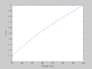
% Now lets go further and calculate it for a bunch of n
n = 30:10:100;
t_stat = (P - p0)./sqrt(p0 * (1-p0)./n);

figure()
plot(n,t_stat)
xlabel('Sample Size')
ylabel('T stat')

% BINGO: We got it. So at a sample Size of 100, we get Exactly what we
% wanted. We REJECT the NULL Hypothesis that It was a TIE and declare A as
% our winner in the survey.

Reverse Experiment: calculating Percentages Needed with a given Sample Size to have statistical significance.

% So here we need to find out for what P value is needed.

% With Some Linear Algebraic Manipulations, we get:

% Now find out for different n , what P is needed..

n = 21:30;
P = p0 + [2 * sqrt(p0 * (1-p0)./n)];

figure()

plot(n,P)

xlabel('Sample Size')

ylabel('Probability Needed to have statistical siginificance')


% For Larger Samples:

n = 30:1000;
P = p0 + [2 * sqrt(p0 * (1-p0)./n)];

figure()

plot(n,P)

xlabel('Sample Size')

ylabel('Probability Needed to have statistical siginificance')

ee How the PLOT flattens out after certain number of Samples( >450).

That is why most of the proffessional Pollsters pick a sample size of Approximately 500

History behind "Rules-of-thumb" (Why 22? 25? 30?)

(Source: iSixSigma)

n=22 was proposed by Fisher in Statistical Mehthod, p. 44, when he reviewed the impact of the the exeeding of the standard deviation once in evey three trials. Twice the standard deviation is exceeded in about 22 trials "For p-value = 0.05, or 1 in 20 and 1.96 or nearly 2; it is convenient to take the point as a limit in judging whether a deviation is to be condisered significant or not. Deviations exceeding twice the standard deviation are thus formally regarded as significant. Using this criterion we should be led to follow up a false indication only once in 22 trials even if the statsitics were the only guide. Small effects will still escape notice if the data are insufficiently numerous to bring them out, but lowering of the standard of signficicance meet this difficulty.

n = 25 has a truly statistical justification. At n = 25 the Law of Large numbers will start to show a pronounced symmetric/normal distribution of the sample means around the population mean. This normal distribution becomes more pronounced as n is increased.

n = 30 comes from a quote from Student (Gosset) in a 1908 paper "On the probable error of a Correlation" in Biometrika. In this paper he reviews the error associated with drawing of two independent samples from infinitely large population and their correlation (not the individual errors of each sample relative to the sample mean and the population mean!). The text reviews
different corrections to the correlation coefficient given various forms of the joint distribution. In a few sentences, Student says that at n = 30 (which is his own experience) the correction factors don't make a big difference.

Later, Fisher showed that the sample for a correlation needs to be determined based on a z-transformation of the correlation. So, Student's argument is only interesting historically. Also, Student wrote his introduction of the t-test in Biometrika during the same year (his
prior article). Historically, the n = 30 discussed in his correlation paper has been confused with the t-test paper, which only introduced the t-statistic up to sample size 10.

References:

1. http://faculty.chicagogsb.edu/jeffrey.russell/teaching/bstats/handouts/notes.pdf

2. http://www.isixsigma.com/

3. http://www.itl.nist.gov/div898/handbook/ppc/section3/ppc333.htm

4. http://www.itl.nist.gov/div898/handbook/prc/section2/prc222.htm

5. http://www.itl.nist.gov/div898/handbook/prc/section2/prc243.htm