Stock Symbol Change History Nasdaq

Symbols of stocks change due to various reason at the exchange.

A quick google check took me to this url :

http://www.nasdaq.com/markets/stocks/symbol-change-history.aspx

The problem was it was 19 pages . There was no easy way to download them all.

So wrote a small snippet of code that goes through each page and downloads it.

The following code gives you a way to download the stock symbols change.

NASDAQ Symbol Change Matlab code

NASDAQ Symbol change history Excel file

CUSIP Lookup

I recently updated my old code that looks up a cusip and gets the symbol from fidelity website.

convert stock cusips to stock symbols

Another way is to directly get the list of cusips from SEC published 13f lists here (in pdf) :

13f lists

ETF Covered Calls - New Blog

I have started a new blog that gives information on ETF covered calls. Here I port an excel sheet that calculates the Covered Call Strategy returns for optionable ETFs.

http://etfcoveredcalls.blogspot.com

ETF Covered Calls

Yahoo Options Data web scraper in matlab

I use Yahoo Option Chains Data to quickly check on the Option prices. I wrote a web scraper that conveniently fetches the Yahoo Option Chain Data into matlab. I hope it will be useful for some people.

UPDATE : I have edited the link below. It seems like the link was blocked for some reason.

Yahoo Options Data

Thanks

Interactive Brokers Product List Web Scraper

I use Interactive Brokers to trade for my personal account. Several times I needed to check the Product list page to get the symbols and other information . I wrote a small program to download it automatically into matlab. Hopefully the readers will find it useful.

The file is available here :
IB_Product_List_Scrapper.m

Pairs Trading--Cointegration Testing

There are several papers on this topic. A quick google search gives you a list of research papers on this topic. Cointegration technique is sometimes used to do Pairs trading. By checking if a pair of stocks are cointegrated, one could go long on one stock and short on the other (multiplied by Hedge Ratio). We are thus trying to be market neutral. Carol Alexander in the book "Market Models" gives a very good explaination of the theory behind it.

A set of I(1) series are termed "cointegrated" if there is a linear combination of these series that is stationary. Stock A and Stock B are cointegrated if A,B are approximately I(1), but there is Hedge Ratio such that

Spread = StockA - Hedge_Ratio * StockB is Approximately I(0). I.e The spread is stationary or mean reverting.

So We perform the following Steps to Check if two stocks are cointegrated:

Step1 : Check if the two stocks are atleast integrated of order 1, I(1)
This is done with Augmented Dickey fuller Test

Step2: After they pass the above test, perform a Cointegration augmented dickey fuller test

Step 3: After it passes the ADF test, we can perform a Ordinary Least Squares Regression to get the Hedge Ratio (The Beta of the regression)

Step 4: So the Spread = StockA - Hedge_Ratio * StockB would now be Cointegrated (mean reverting)

Step 5: Figuring when to exit : Calculate Half Life

Half life basically tells you how much time it takes for the spread to revert back to half the distance of the mean.

Step 6: Calculate the Spread TODAY. Calculate the Standard deviation of the spread upto the day before. Check how far the current spread is from the historical average. If it is greater than 1.5 standard deviations (or any other threshold), then go short the spread otherwise go long the spread. I.e Go Short Stock A and Long Hedge Ratio * Stock B. Be in the trade until the half life calculated for the pair. If the Half Life time period has passed, Get out of the trade.

These are simple steps. One should put on more work and research on it to develop it into a practical trading strategy.

Some interesting papers are here:

Cointegration Paper I

Cointegration Carol Alexander


MATLAB Code Here:

MATLAB COINTEGRATION CODE

CointPairsTrade.m is the main function and calls all other functions

Please let me know if there are any bugs

Calculating Implied Dividend Yield from Option Prices

Here is the formula that one could use to calculate the Implied dividend yield:

PV(Dividend) = -CALL + PUT + (Spot - Strike) + ((Strike * exp(r*T)) - Strike)

where r is the interest rate to expiration. T is the time to maturity in Years.

Implied Dividend Yield = PV(Dividend)/(T * Spot)

Taking the Example of PFE, Pfizer Inc

Taking the Option prices of June 2010 Expiration

Spot = 18.49
CALL = 1.72
PUT = 1.52
r = 0.16%
T = 0.5 (Approx)
ATM Strike = 18

Substituting the above values into the equation below:

PV(Div) = -1.72 + 1.52 + (18.49-18)+ ((18 * exp(0.0016*0.5))-18)

PV(Div) = 0.3044

Implied Dividend Yield = 0.3044/(0.5 * 18.49) = 0.0329 = 3.29%

To Express an opinion that the dividend yield will be reduced, one should go long PFE June 2010 18 CALL, Short one June 2010 18 PUT, and SHORT 100 shares of PFE stock.

To Express an opinion that the dividend yield will be increased, one should go short PFE June 2010 18 CALL, long one June 2010 18 PUT, and long 100 shares of PFE stock.

A simple way to Backtest Option Straddles

Here, I show how one could follow a simple approach to backtest the profitability of Option Straddles. Straddles are a way to get exposure to volatility of a stock. A Long Straddle means buying an AT-THE-MONEY CALL and PUT option of the same expiration date. Vice versa for a Short Straddle position.

TO profit from a straddle position, One should be able to calculate, historically, how many times did the stock move beyond the premium one would pay for the STRADDLE Position. For example, If a Straddle on a stock costs $4, It makes sense to check how many times in the past did the stock move more than $4, UP or DOWN. I.e if the option expires in 30 days, one needs to find out on any given 30 days in the past, how many times has the stock moved beyond $4. This is only one of the many things one needs to do before buying or selling straddles. This combined with the Volatility Cones and calculation of "Average" spread between Realized Volatility and Implied Volatility should give an investor some information to trade them. One can also look into "Strangle".

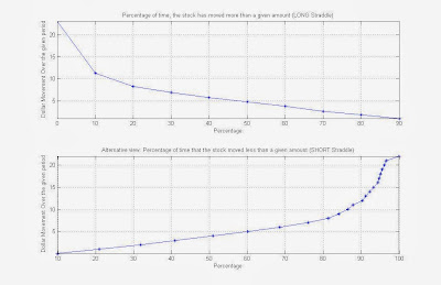
Here is a figure that shows a stocks historical movements over the past 3 years for a 30 day rolling window period.


One can see from the chart that in the past 3 years, CNH has moved beyond $5 only 50% of the time, 60% more than $3.8, 70% more than $2.66 etc. So if a straddle costs only $2.66, then Historically, 70% of the time it has moved more than $2.66 in 30 days. On the other side, there is still a 30% chance that it will not move beyond $2.66.




MATLAB CODE:

Backtest_Straddles.m

Using Volatility Cones

This post describes what volatility cones are and how I usually use them. As with many of my posts, I will attach code to this post.

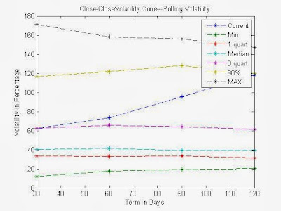
Volatility cones are a graphical representation of realized volatility ranges over different time horizons such as 30,60,90,120 days. It gives a volatility distribution. It puts the current implied volatility into perspective. Some quotes from the book volatility trading by euan sinclair :

" The volatility cone is very useful for placing current market information (realized volatility, implied volatility and the spread between them) into historical context.We may be best served by comparing implied volatility to the historical volatility distribution given by the volatility cone. Selling one-month implied volatility at 35% because this is in the 90th percentile for one-month volatility over the past 2 years can form the basis of a sensible trading plan."

One needs to calculate the spread between 30 day rolling close to close volatility and the Implied Volatility. One needs to calculate the AVERAGE of the above spread over a sufficient time period. If the spread is Above normal then one needs to look carefully as an opportunity to trade.

As an Example, The above plot shows the Volatility cone of stock : CNH as of today 06/29/2009

The 30, 60, 90, and 120 day rolling volatilities and their percentiles are shown below and plotted above in the figure.

30 60 90 120
-----------------------------------
Current: 0.6252 0.7363 0.9564 1.1798
Min: 0.1205 0.177 0.19 0.2023
25% : 0.3324 0.3301 0.3318 0.3149
50% : 0.4039 0.4118 0.3943 0.3924
75%: 0.6239 0.6538 0.639 0.6148
90%: 1.1666 1.2162 1.2797 1.1961
MAX: 1.7115 1.5827 1.5581 1.4694


As you can see from the above table, CNH 60 day volatility has varied from a minimum of 17.7% to a maximum of 158%. The close price today is $14.32. The nearest Strike for 08/22/2009 Expiration is $15. The Implied Volatility of the call Option is 69.5 ( from Options Express website). The number of days to Expiry is 53. The Implied vol of 69.5 falls between 75% to 90% . So Approx 80% of the time in the past 4 years, the Realized Volatility of 60 days has been below that number of 69.5%. So we are in the third quartile. Whether this is high enough to sell the implied volatility or not depends on the person's risk appetite. This information gives me confidence in making the trade intelligently.

Code:

Please download all the three files into the same directory and run VolCones_CC.m

VolCones_CC.m


EstimateVol_CC.m


hist_stock_data.m

VIX vs S&P 500 Expected Returns Range

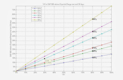
In this post, I give out a ready to use figure or plot that one could keep handy to relate VIX level to the Expected S&P 500 returns Range over the next 30 days. I also show how the plot is derived. DOUBLE CLICK THE PLOT FOR A BIGGER IMAGE

As you can see from the Above figure, one can easily figure out the expected range of S&P 500 Returns with a given VIX Level for a given Probability. For example, Currently the VIX level is 30%. So looking at the above plot, for 90% Probability,30% VIX,on the X-Axis and following it vertically and across, we can see that over the next 30 days, the expected range for S&P 500 Returns is +/- 14.24% .

In general, The linear relationship is as follows:

Expected Range with 50% Probability = 0.1947 * VIX

Expected Range with 68% Probability = 0.2871 * VIX

Expected Range with 75% Probability = 0.3321* VIX

Expected Range with 90% Probability = 0.4748* VIX

Expected Range with 95% Probability = 0.5658 * VIX

Expected Range with 99% Probability = 0.7436 * VIX

Now I show how I derived the Above Plot

% probabilities
p = [0.50 0.68 0.75 0.90 0.95 0.99]
% Properly adjust those probabilities to be passed into norminv program
p2 = 0.50 + p./2;

% Before we proceed we should make an important assumption that
% The rate of return on the S&P 500 over the next 30 days is normally
% distributed

% USe the norminv command to get the number of standard deviations
% that a number drawn from unit normal distribution will be

nstd = norminv(p2,0,1);

% since VIX is is an annualized standard deviation, We divide the values
% Obtainded above by sqrt(12)

nstd = nstd ./ sqrt(12);

% Now the Linear Relationship between Level of VIX and S&P 500 return range
% would be: ExpRangeSP500 = nstd .* VIX
% Now let us plot using various values of VIX

VIX = 0:10:100;
ExpRangeSP500 = nstd' * VIX;

%%PLOT
plot(VIX,ExpRangeSP500,'-*')
set(gca,'YTick',[0:5:max(ExpRangeSP500(:))])
set(gca,'YtickLabel',cellstr(strcat(num2str([0:5:max(ExpRangeSP500(:))]'),'%')))
set(gca,'XTickLabel',cellstr(strcat(num2str(VIX'),'%')))
title('VIX vs S&P 500 returns Expected Range over next 30 days')
xlabel('VIX')
ylabel('S&P 500 returns Expected Range over next 30 days')
plottitles = strcat(cellstr(num2str(p' .*100)),'%');
legend(plottitles,'Location','best')
text(VIX(9)*ones(6,1),ExpRangeSP500(:,9),plottitles,'FontSize',14,'FontWeight','bold')
grid on
axis tight

Applying VIX methodology to Stocks (American )

GOOGLEDOCS file:

http://docs.google.com/View?id=ddb2j6dw_13dg24q4mk




In this post I show how one could utilize the VIX methodology for American
Options.VIX was designed with European Type Options. It was designed
for S&P500 Options ( which are European ). But when applied to American
Options,These have a bias due to early exercise and Dividend and disbursement
events. If the forecasted period avoids dividends, then the bias should
be minimal. Neverthelss, It can be used as a valuable forecast or a
technical indicator.


function VIX = ReplicateVixStock(Data,TM,Rf,CT)
%REPLICATEVIXSTOCK applies VIX methodology for stocks (American Options)
% VIX was designed with European Type Options. It was designed for S&P500
% Options ( which are European ). But when applied to American Options,
% These have a bias due to early exercise and Dividend and disbursement
% events. If the forecasted period avoids dividends, then the bias should
% be minimal. Neverthelss, It can be used as a valuable forecast or a
% technical indicator.
% Inputs: If NO Inputs are provided, Example will run
% Data: Should be cell array with separate data for two Maturities
% centered around 30 days. I.e One option expiry must be less than 30
% days and the other should be greater than 30 days.
% Data is a three column data with Strike, Call and Put Prices.
% Data{1} should be Near Term Option Data
% Data{2} should be far Term Option Data
% TM : Time to maturity for two options
% Rf : Risk free Rate
% CT : Current Time ( Time Stamp when The data was collected )
% Output : VIX-- A single number that Applies the VIX methodology to the
% American Options
% Example : Try running with NO inputs

if(nargin==0)
% Near-Term
% Strike Call Put
Data{1} = [75 11.75 0.05;...
80 6.90 0.08;...
85 2.40 0.60;...
90 0.18 3.40;...
95 0.05 8.30;...
];

% Next Term
% Strike Call Put
Data{2} = [75 NaN NaN;...
80 7.70 0.73;...
85 3.80 1.80;...
90 1.05 4.05;...
95 NaN NaN;...
];
%Time_To_Maturity
TM = [9;37];
%Risk_Free_Rate
Rf = 1.1625/100; %Per Annum
% Current Time
CT = '12:09:00';
end

% remove NaN Rows
Data{1}((any(isnan(Data{1}),2)),:)=[];
Data{2}((any(isnan(Data{2}),2)),:)=[];

% Difference between Calls and Puts (Absolute Value)
DF{1} = abs(Data{1}(:,2) - Data{1}(:,3));
DF{2} = abs(Data{2}(:,2) - Data{2}(:,3));

% FInd Hour, Minute, Second from the time using datevec function
[Year, Month, Day, Hour, Minute, Second] = datevec(CT);
%In Years
%1440 is the number of minutes in a day and 510 is the number
% of minutes to 8:30 AM which is the time the option expires
% on its expiration date
NumYears(1) =[1440 - (Hour * 60 + Minute + Second/60) + 510]/ ...
(1440 * 365) + [(TM(1) - 2)/365];
NumYears(2) =[1440 - (Hour * 60 + Minute + Second/60) + 510]/ ...
(1440 * 365) + [(TM(2) - 2)/365];
% In days
NumDays = NumYears .* 365;
% Find the minimum of the difference in Call and Put
% Prices and Get the corresponding Strike Price.
ATM(1,:) = Data{1}((DF{1}==min(DF{1})),:);
ATM(2,:) = Data{2}((DF{2}==min(DF{2})),:);
% Calculate Forward Price Level and Referential Strike
% Application of PUT CALL Parity
Level = ATM(:,1) + exp(Rf*NumYears(:)) .* (ATM(:,2) - ATM(:,3));
%Reference Strike
for i = 1:2
Strike = ATM(i,1);
if(ATM(i,2)>=ATM(i,3))
Ref_Strike(i)=ATM(i,1);
else
Ref_Strike(i) = Data{i}(find(Data{i}(:,1) < ATM(i,1),1,'last'),1);
end
% Differences of Strikes
Temp = diff(Data{i}(:,1));
Delta_Strike{i} = [Temp(1);Temp];

% If the strike is above the “reference strike” , use the call price
% If the strike is below the “reference strike” , use the put price
%If the strike equals the “reference strike” , use the average of the call
% and put prices

cpval= zeros(size(Data{i},1),1);
cid = find(Data{i}(:,1) > Ref_Strike(i));
cpval(cid) = Data{i}(cid,2);
pid = find(Data{i}(:,1) < Ref_Strike(i));
cpval(pid) = Data{i}(pid,3);
Aid = find(Data{i}(:,1) == Ref_Strike(i));
cpval(Aid) = (Data{i}(Aid,2) + Data{i}(Aid,3))/2;

% Now do the math as given in the paper vixwhite.pdf

vix{i} = Delta_Strike{i} * exp(Rf*NumYears(i)) .* cpval ./(Data{i}(:,1).^2);
Var(i) = (2/NumYears(i)) * sum(vix{i}) - ((Level(i)/Ref_Strike(i) ...
- 1).^2)/NumYears(i);

% Center the data to 30 days
if(i==1)
Term(i) = NumYears(i) * Var(i) * ((NumDays(i+1)-30)/(NumDays(i+1)-NumDays(i)));
elseif(i==2)
Term(i) = NumYears(i) * Var(i) * ((-NumDays(i-1)+30)/(NumDays(i)-NumDays(i-1)));
end


end %i

% Final Vix Calculation
VIX = sqrt(sum(Term) * 365/30) * 100;

Search for Covered Calls and also Build Options data Database

This post is in continuation to my previous blog post on getting the Options Data from websites such as Yahoo, Optionetics and Options Express. I wanted to collect End-Of-Day Options Data from those websites and search for Covered Calls that I could trade. Covered Call is a strategy wherein you buy the stock and write an Out-of-the money CALL option and thus generate monthly income from the stock. This strategy can also be used if you already own a stock and want to earn some income on it. You can also write In the Money Call Option which will give you more downside protection, but less return. At the end of each day one can run the following program and thus store the options Data and use it for further analysis.

After collecting the data, One could search for those stocks that have the highest premium and which you think are good stocks and wont mind holding on to them.


Note that this function depends on Get_Yahoo_Options_Data2.m function that I talked about in my previous blog post. One can purchase it, if interested.

%%%%%%%%%% CODE %%%%%%%%%%%%%%%%

function Out = CoveredCalls(SymbolList)
%CoveredCalls gives the Options Data and Calculates Covered Calls returns
%for a given Symbol for that particular day
% This function can also be used to build a database of Options Data
% on a daily basis.
% NOTE that This function requires Get_Yahoo_Options_Data2.m function

% Inputs: A cell array of Symbols
% Output: A structure with the following fields:
% calldata : This contains the Calls data and also has Flat and
% Exercised returns
% The colummn names are as follows:
% {'Symbol','Strike','Last','Change','Bid','Ask','Volume','Open Int',
% 'Expiry','MonthNum','time Value','Exercise Return','Flat Return'};
% RawData : This contains Both the Calls and Puts Data
% The column names are as follow:
% {'Symbol','Last','Change','Bid','Ask','Volume','Open Int','Strike',
% 'Symbol','Last','Change','Bid','Ask','Volume','Open Int',
% 'Expiry','MonthNum','Last Price'};

% Example:
% Out = CoveredCalls({'cnh','ibm'});
% If user wants a single big cell array, one can get it by using command:
% vertcat(Out.calldata{:})

% (c) tradingwithmatlab.blogspot.com

% Atleast one input is required
if(nargin < 1)
error('Atleast one Input is needed')
end
% Check if its either a cell array or Character
if~(ischar(SymbolList)||iscell(SymbolList))
error('SymbolList needs to be either a character or Cell Array')
end

if(iscell(SymbolList) && ~isvector(SymbolList))
error('SymbolList needs to be a cell array')
end

% Convert Char to a cell string
SymbolList = cellstr(SymbolList);

% Number of Symbols
nsymbols = length(SymbolList);
% Initialize
Out.calldata = cell(nsymbols,1);
Out.RawData = cell(nsymbols,1);

% for each symbol, Get the Options Data and Calculate The returns

for idx = 1:nsymbols;idx
% Get Data from YAHOO
data = Get_Yahoo_Options_Data2(SymbolList{idx});
% We are interested only in CALL options

calldata = data.Calls;
LastPrice=data.Last;

if(isempty(calldata))
continue
end
% Get the Parameters
Strike = cell2mat(calldata(:,2));
Bid = cell2mat(calldata(:,5));
LastPrice = LastPrice(ones(length(Bid),1));

% Calculate Time value---If Option Exercised
TimeValue = Strike + Bid - LastPrice;
TimeValuePercent = TimeValue./LastPrice;

% Calculate Flat return
FlatReturn = Bid ./ LastPrice;

% Store the data
Out.calldata{idx} = [repmat(SymbolList(idx),size(calldata,1),1),...
calldata num2cell([TimeValue TimeValuePercent FlatReturn])];

Out.RawData{idx} = [data.data num2cell(LastPrice)];
end

Convert Stock CUSIPs to Stock Symbols with a MATLAB program

UPDATE : Thanks to a comment, I changed the code to reflect the new changes at fidelity site.

CUSIP is a 9 character(alpha-numeric ) identifier. It actually stands for "Committee on Uniform Security Identification Procedures". Sometimes it is very useful to be able to look up the Stock Symbol that the CUSIP represents. I had a list of CUSIPS and some data associated with it. I did not have the Stock Symbols Associated with Them. I was only interested in Stock CUSIPS. I searched online and found out that there was no automated way of finding out the stock symbol associated with stock CUSIPS. So I wrote the following program to look up the CUSIP at the Fidelity website and grab the stock symbol associated with it. I extensively used regular expressions. I hope this program will be useful to others.

For example:
'031162100' given Amgen Inc---AMGN
Symbols = CusipToSymbolLookUp({'031162100';'03116210';})

function Symbols = CusipToSymbolLookUp(Cusip)
%CUSIPTOSYMBOLLOOKUP converts STOCK CUSIPS to STOCK Symbols
% Symbols = CusipToSymbolLookUp(Cusip) gives a list of STOCK symbols that
% correspond to a list of Cusips.
% This function looks up a STOCK symbol for a given CUSIP
% The CUSIP needs to be 8 or 9 characters long
% If a valid 8 character Cusip is given, then a 9th check digit is added if
% possible.It accesses the fidelity website and does html parsing
% to get the symbol name. Cusip can be a cell array of Cusips
% More information on CUSIPs can be found at:
% http://www.cusip.com
% I Thank Nabeel Azar for his program checkcusip.m
% Example:
% Symbols = CusipToSymbolLookUp({'031162100';'03116210';})

% Atleast one input is required
if(nargin < 1)
error('Atleast one Input is needed')
end
% Check if its either a cell array or Character
if~(ischar(Cusip)||iscell(Cusip))
error('Cusip needs to be either a character or Cell Array')
end

if(iscell(Cusip) && ~isvector(Cusip))
error('Cusip needs to be a cell array')
end

% Convert Char to a cell string
Cusip = cellstr(Cusip);

% Find how many cusips were given
ncusips = length(Cusip);

% Intial Web URL
weburl = ['http://activequote.fidelity.com/mmnet/SymLookup.phtml?reqforlookup=REQUESTFORLOOKUP&productid=mmnet&isLoggedIn=mmnet&rows=50&for=stock&by=cusip&criteria='];

% Pre assign the Output
Symbols = cell(ncusips,1);

% Now go through the List and do the processing
for idx = 1:ncusips

% If The Length of the Cusip is 8 digits/characters long,
% Then It is converted into 9 digits using a program called checkcusip
% If it returns a logical false, then it is a wrong CUSIP
% If it returns a double digit, then join the checkdigit to the
% original CUSIP

if(length(Cusip{idx})==8)
Result = checkcusip(Cusip(idx));
if (islogical(Result{1}) && Result{1}==false)
continue
else
% Join the Cusip with CheckDigit
Cusip{idx} = [Cusip{idx} num2str(Result{:})];
end

% If the Length is not equal to 9, then just continue
elseif(length(Cusip{idx})~=9)
continue
end

% Construct the URL using the Cusip and read the url
%[weburl Cusip{idx} '&submit=Search']
data = urlread([weburl Cusip{idx} '&submit=Search']);


% Search for a preliminary pattern
%pat = '<(a HREF).*?>.*?';
pat = 'SID_VALUE_ID=([a-zA-Z]+)">';

% Use regexp to match the pattern
data2=regexp(data,pat,'tokens');

% Use another pattern to get the symbol
if(~isempty(data2))
% pat = '>\w*<';
% sname=char(regexp(data2{1},pat,'match'));
Symbols(idx) = data2{1};
end

% % Pre-Process the Output before storing it in an array
% if(~isempty(sname))
% sname([1 end])='';
% Symbols{idx} = sname;
% end

end


function Result = checkcusip(inputCell)
%CHECKCUSIP Check a CUSIP
% CHECKCUSIP is used to validate 9 digit CUSIPs and
% provide the checkdigit for 8 digit CUSIPs.
%
% Note that if you give this function a combination of
% 8 and 9 digit CUSIPs, you need to check both the class
% (logical or non-logical) as well as the value of the
% output. Logicals are used to indicate validity of a
% 9 digit CUSIP, while non-logical doubles are used to
% supply the checkdigit for an 8 digit CUSIP.

% Convert the input to a char array
if iscell(inputCell)
cusipCharArray = strvcat(inputCell{:});
else
error(['Inputs must be cell arrays of CUSIP strings.'])
end


% Make sure there are at least 8 columns
if size(cusipCharArray,2)<8 p="">error(['Must supply 8 or 9 digit CUSIPs.']);
end

% Make them all lowercase
cusipCharArray = lower(cusipCharArray);




%%%%%%%%%%%%%%%%%%%%%%%%%%%%%%%%%%%%%%%%%%%%%%%%%%%%%%%%%%%%%%%
% Convert the string digits to numerical values and
% the characters to their numerical values, with 'A':=10
% Set spaces (for computing the checkdigit) to NaNs

% Transpose the array, and work down the columns.
longCusipString = double(cusipCharArray);
longCusipString = longCusipString.';
numericalLocations = (longCusipString>='0' & longCusipString<='9');
charLocations = (longCusipString>='a' & longCusipString<='z');
NaNLocations = longCusipString==' ';

longCusipString(numericalLocations) = longCusipString(numericalLocations) - '0';
longCusipString(charLocations) = longCusipString(charLocations) - 'a' + 10;
longCusipString(NaNLocations) = NaN;

% Get the cusip digits
cusipNums = longCusipString(1:8,:);

% Scale with scaling factors
cusipNums = diag([1 2 1 2 1 2 1 2]) * cusipNums;

% Sum the digits in each term >=10;
gt_10 = cusipNums>=10;
cusipNums(gt_10) = floor(cusipNums(gt_10)/10) + rem(cusipNums(gt_10),10);

% Sum the resulting values
cusipNums = sum(cusipNums);

% Get the last digit
lastDigit = rem(cusipNums,10);

% Generate the checkdigit
checkDigit = 10 - lastDigit;
checkDigit(checkDigit==10) = 0;

%%%%%%%%%%%%%%%%%%%%%%%%%%%%%%%%%%%%%%%%%%%%%%%%%%%%%%%%%%%%%%%%%


% Create a cell array the right size for the output.
Result = cell(numel(inputCell),1);

% If no check digit was given in the input, output the checkdigit
if size(longCusipString,1)==9
needCusip = isnan(longCusipString(9,:));
else
needCusip = logical(ones(1,size(longCusipString,2)));
end
Result(needCusip) = num2cell(checkDigit(needCusip));

% If a check digit was given, validate it
if size(longCusipString,1)==9
isCheckdigitCorrect = longCusipString(9,~needCusip)==checkDigit(~needCusip);
Result(~needCusip) = num2cell(isCheckdigitCorrect);
end

% Only the 1st, 4th, 5th, or 6th digit may be an alphanumeric letter
% (1st for international issues)
badIdx = any(longCusipString([2 3 7 8],:)>=10,1);
Result(badIdx) = {logical(0)};

% The first digit cannot be an i, o, or z
badIdx = any(longCusipString(1,:)=='i' | longCusipString(1,:)=='o' | longCusipString(1,:)=='z',1);
Result(badIdx) = {logical(0)};

% Reshape the result
Result = reshape(Result,size(inputCell));

Replicate VIX (CBOE Volatility Index) --MATLAB Implementation

This post is just to demonstrate how to replicate the Calculations behind the CBOE Volatility Index, Commonly called VIX. It is also commonly thought of investor gauge of fear. One can read more about at www.cboe.com

The Implementation below follows the methodology as illustrated in the following white paper:

http://www.cboe.com/micro/vix/vixwhite.pdf

M FILE is here:

http://docs.google.com/Doc?id=ddb2j6dw_12fjk57bfx




CODE Published Here:

%% ReplicateVIX
% Near-Term
% Strike Call Put
Data{1} = [775 125.48 0.11;...
800 100.79 0.41;...
825 76.70 1.30;...
850 54.01 3.60;...
875 34.05 8.64;...
900 18.41 17.98;...
925 8.07 32.63;...
950 2.68 52.33;...
975 0.62 75.16;...
1000 0.09 99.61;...
1025 0.01 124.52];
% Next Term
% Strike Call Put
Data{2} = [775 128.78 2.72;...
800 105.85 4.76;...
825 84.14 8.01;...
850 64.13 12.97;...
875 46.38 20.18;...
900 31.40 30.17;...
925 19.57 43.31;...
950 11.00 59.70;...
975 5.43 79.10;...
1000 2.28 100.91;...
1025 0.78 124.38];

%Time_To_Maturity
TM = [16;44];
%Risk_Free_Rate
Rf = 1.1625/100; %Per Annum
% Difference between Calls and Puts (Absolute Value)
DF{1} = abs(Data{1}(:,2) - Data{1}(:,3));
DF{2} = abs(Data{2}(:,2) - Data{2}(:,3));
% Current Time
CT = '08:30:00';
% FInd Hour, Minute, Second from the time using datevec function
[Year, Month, Day, Hour, Minute, Second] = datevec(CT);
%In Years
%1440 is the number of minutes in a day and 510 is the number of minutes to 8:30 AM which
%is the time the option expires on its expiration date
NumYears(1) = [1440 - (Hour * 60 + Minute + Second/60) + 510]/(1440 * 365) + [(TM(1) - 2)/365];
NumYears(2) = [1440 - (Hour * 60 + Minute + Second/60) + 510]/(1440 * 365) + [(TM(2) - 2)/365];
% In days
NumDays = NumYears .* 365;
% Find the minimum of the difference in Call and Put
% Prices and Get the corresponding Strike Price.
ATM(1,:) = Data{1}(find(DF{1}==min(DF{1})),:);
ATM(2,:) = Data{2}(find(DF{2}==min(DF{2})),:);
% Calculate Forward Price Level and Referential Strike
% Application of PUT CALL Parity
Level = ATM(:,1) + exp(Rf*NumYears(:)) .* (ATM(:,2) - ATM(:,3));
%Reference Strike
for i = 1:2
Strike = ATM(i,1);
if(ATM(i,2)>=ATM(i,3))
Ref_Strike(i)=ATM(i,1);
else
Ref_Strike(i) = Data{i}(find(Data{i}(:,1) < ATM(i,1),1,'last'),1);
end
% Differences of Strikes
Temp = diff(Data{i}(:,1));
Delta_Strike{i} = [Temp(1);Temp];
%{
? If the strike is above the “reference strike” , use the call price
? If the strike is below the “reference strike” , use the put price
? If the strike equals the “reference strike” , use the average of the call
and put prices
%}
cpval= zeros(size(Data{i},1),1);
cid = find(Data{i}(:,1) > Ref_Strike(i));
cpval(cid) = Data{i}(cid,2);
pid = find(Data{i}(:,1) < Ref_Strike(i));
cpval(pid) = Data{i}(pid,3);
Aid = find(Data{i}(:,1) == Ref_Strike(i));
cpval(Aid) = (Data{i}(Aid,2) + Data{i}(Aid,3))/2;

% Now do the math as given in the paper vixwhite.pdf

vix{i} = Delta_Strike{i} * exp(Rf*NumYears(i)) .* cpval ./(Data{i}(:,1).^2);
Var(i) = (2/NumYears(i)) * sum(vix{i}) - ((Level(i)/Ref_Strike(i) - 1).^2)/NumYears(i);

% Center the data to 30 days
if(i==1)
Term(i) = NumYears(i) * Var(i) * ((NumDays(i+1)-30)/(NumDays(i+1)-NumDays(i)));
elseif(i==2)
Term(i) = NumYears(i) * Var(i) * ((-NumDays(i-1)+30)/(NumDays(i)-NumDays(i-1)));
end


end

% Final Vix Calculation
VIX = sqrt(sum(Term) * 365/30) * 100

Sample Size Determination and History behind Rules of Thumbs( Why 22? Why 25? Why 30?)

Sample Size equation that is predicated on Central Limit Theorem

• Correction Factor for Sample Size based on finite Population Size

Plot of SampleSize Required vs Probability:

T-distribution table VS Sample Size and closeness to Standard Normal:

Survey Example: Some tests for Sample Sizes:

NULL HYPOTHESIS:

T-stat formula

Reverse Experiment: calculating Percentages Needed with a given SampleSize to have statistical significance.

• History behind "Rules-of-thumb" (Why 22? 25? 30?)

References:

Sample Size equation that is predicated on Central Limit Theorem

Correction Factor for Sample Size based on finite Population Size

For a 95% Level, Z = 1.96. Let us say that we want the result to be within 5% error--Confidence Interval and lets have P varying
from 0.1 to 0.9. Then inserting the above numbers into the equation, we get:
ConfidenceInterval = 0.05;Z = 1.96;

P = 0.1:0.1:0.9;
SampleSize = [Z^2 .* P .* (1-P)]/(ConfidenceInterval^2);
SampleSizeRequired = [P ;SampleSize].'
SampleSizeRequired =
0.1000 138.2976
0.2000 245.8624
0.3000 322.6944
0.4000 368.7936
0.5000 384.1600
0.6000 368.7936
0.7000 322.6944
0.8000 245.8624
0.9000 138.2976

Plot of SampleSize Required vs Probability:

figure()

plot(SampleSizeRequired(:,1),SampleSizeRequired(:,2))

xlabel('Probability P')

ylabel('Sample Size Required')

T-distribution table VS Sample Size and closeness to Standard Normal:

(Source: Jeffrey Russell NOTES)

T distribution with n-1 degrees of freedom at 0.05 level( 95%) It becomes normal when T is Approx 2 ( 1.96 to be exact)

% T     n

[4.303   3
2.228   11
2.086   21
2.042   31
2.00    61];

% As can be seen above Starting from about 21 we can see it get closer to 2

Survey Example: Some tests for Sample Sizes:

(Source: Jeffrey Russell NOTES)

Assume IID (Independent Identical distribution). So now let us say we
need to do a survey. Let us assume that we have
ONLY 21 (From the above Table) people to survey from.

After survey we found that 60% People say A and 40% say B. Now We need to find out if it is significant or not. We need to find out by calculating

% the T-stat and comparing it with 2 (1.96 to be exact).

NULL HYPOTHESIS:

IT IS TIE (50-50). I.e Even though 60% of the people say A, we want to make sure it is different from being a TIE (50-50)
when a bigger population is considered.

T-stat formula ( Any Basic Stats Textbook is the source here)

T_Stat = (P - p0)/sqrt(p0 * (1-p0)/n); Where p0 is NULL hypothesis. (0.50 in our case)

% Now lets put some values into the equation:

P = 0.60; p0 = 0.50;%( NULL Hypothesis)
n = 21;
t_stat = (P - p0)/sqrt(p0 * (1-p0)/n)

t_stat = 0.9165

% We GOT 0.9165 Which is LESS than 2. So we FAIL to reject the NULL
% Hypothesis. So we cannot say with certainty that it is NOT a TIE.

% Now lets increase the n to 30.
n=30;
t_stat = (P - p0)/sqrt(p0 * (1-p0)/n)

t_stat = 1.0954

% We GOT 1.0954 Which is STILL LESS than 2. So we FAIL to reject the NULL
% Hypothesis. So we cannot say with certainty that it is NOT a TIE.

% Now lets go further and calculate it for a bunch of n
n = 30:10:100;
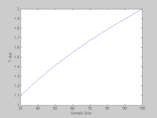
t_stat = (P - p0)./sqrt(p0 * (1-p0)./n);

figure()
plot(n,t_stat)
xlabel('Sample Size')
ylabel('T stat')

% BINGO: We got it. So at a sample Size of 100, we get Exactly what we
% wanted. We REJECT the NULL Hypothesis that It was a TIE and declare A as
% our winner in the survey.

Reverse Experiment: calculating Percentages Needed with a given Sample Size to have statistical significance.

% So here we need to find out for what P value is needed.

% With Some Linear Algebraic Manipulations, we get:

% Now find out for different n , what P is needed..

n = 21:30;
P = p0 + [2 * sqrt(p0 * (1-p0)./n)];

figure()

plot(n,P)

xlabel('Sample Size')

ylabel('Probability Needed to have statistical siginificance')


% For Larger Samples:

n = 30:1000;
P = p0 + [2 * sqrt(p0 * (1-p0)./n)];

figure()

plot(n,P)

xlabel('Sample Size')

ylabel('Probability Needed to have statistical siginificance')

S

ee How the PLOT flattens out after certain number of Samples( >450).

That is why most of the proffessional Pollsters pick a sample size of Approximately 500

History behind "Rules-of-thumb" (Why 22? 25? 30?)

(Source: iSixSigma)

n=22 was proposed by Fisher in Statistical Mehthod, p. 44, when he reviewed the impact of the the exeeding of the standard deviation once in evey three trials. Twice the standard deviation is exceeded in about 22 trials "For p-value = 0.05, or 1 in 20 and 1.96 or nearly 2; it is convenient to take the point as a limit in judging whether a deviation is to be condisered significant or not. Deviations exceeding twice the standard deviation are thus formally regarded as significant. Using this criterion we should be led to follow up a false indication only once in 22 trials even if the statsitics were the only guide. Small effects will still escape notice if the data are insufficiently numerous to bring them out, but lowering of the standard of signficicance meet this difficulty.

n = 25 has a truly statistical justification. At n = 25 the Law of Large numbers will start to show a pronounced symmetric/normal distribution of the sample means around the population mean. This normal distribution becomes more pronounced as n is increased.

n = 30 comes from a quote from Student (Gosset) in a 1908 paper "On the probable error of a Correlation" in Biometrika. In this paper he reviews the error associated with drawing of two independent samples from infinitely large population and their correlation (not the individual errors of each sample relative to the sample mean and the population mean!). The text reviews
different corrections to the correlation coefficient given various forms of the joint distribution. In a few sentences, Student says that at n = 30 (which is his own experience) the correction factors don't make a big difference.

Later, Fisher showed that the sample for a correlation needs to be determined based on a z-transformation of the correlation. So, Student's argument is only interesting historically. Also, Student wrote his introduction of the t-test in Biometrika during the same year (his
prior article). Historically, the n = 30 discussed in his correlation paper has been confused with the t-test paper, which only introduced the t-statistic up to sample size 10.

References:

1. http://faculty.chicagogsb.edu/jeffrey.russell/teaching/bstats/handouts/notes.pdf

2. http://www.isixsigma.com/

3. http://www.itl.nist.gov/div898/handbook/ppc/section3/ppc333.htm

4. http://www.itl.nist.gov/div898/handbook/prc/section2/prc222.htm

5. http://www.itl.nist.gov/div898/handbook/prc/section2/prc243.htm